HadISD Tutorial One - Introduction to Station Data

Hardware Requirements

These tutorials have been tested on a laptop with 36GB of RAM as well as on an HPC node with a large amount of RAM. They do not require a GPU as they do not include model training. 29GB of data will be downloaded. Additional disk space is needed for reprocessing the data. The notebooks may require user modification to run with less than 36GB of RAM.

Overview of HadISD Tutorials

This tutorial is the first of a five-part series dealing with (a) integrating a new data source into PyEarthTools and (b) also forming an introduction to working with station data, an important source of earth system information for model training and evaluation.

For these tutorials, we will use the HadISD dataset. However, the patterns are repeatable, so can be used with other datasets.

The tutorials must be completed in the following order as they implement a series of data processing steps:

1. HadISD Tutorial One - Introduction to Station Data (this tutorial)

2. HadISD Tutorial Two - Downloading the HadISD Dataset

3. HadISD Tutorial Three - Chunking the Data into Small Groups

4. HadISD Tutorial Four - Make Large Groupings

5. HadISD Tutorial Five - Integration of Station Data with PyEarthTools

These tutorials will cover the following:

• Downloading the data in the form distributed by the Hadley centre

• Manually unpacking the data on disk for efficiency reasons

• Re-processing the station data to break it up by decade for file size reasons

• Grouping of individual stations into large station groupings to reduce the number of files on disk

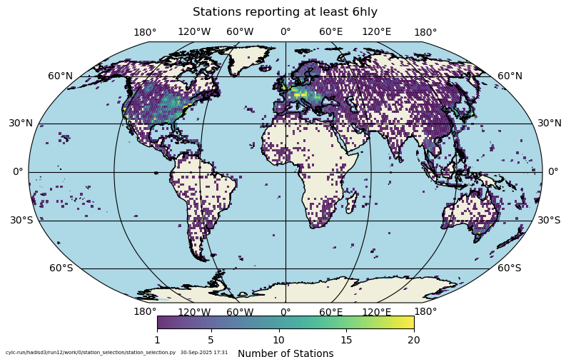
• Data visualisation of the global station data to demonstrate what it looks like following the data restructure

• Integration of this data into a PyEarthTools data accessor

• Integration of station data into a PyEarthTools pipeline

• (to be done) Presentation of gridded data and station data to a neural network for training and prediction

Introduction to Station Data with the HadISD Dataset

Earth system data tends to be either (a) gridded (such as model data, satellite data and radar data) or (b) station-based, such as automated weather stations, weather balloons, floating buoys or airborne observations (i.e. aeroplanes).

Translating between the ‘gridded world’ (e.g. global and regional modelling) and the ‘station world’ is often done by performing a site-based forecast based on gridded inputs (e.g. siteboost or model output statistics). The translation of station data to a gridded model is done through data assimilation. These two ways of working with the data have significant implications for the data structures which will be used, and for computational efficiency. It would be really nice to have a simple API which could abstract away the messy choices, implement the tricky bits and make it easy to just ‘get what we want’.

From a PyEarthTools perspective based on wanting to develop model architectures which include both gridded and point data at the same time (rather than having a ‘translation step’), this means getting the data into a structure where the primary index is date-and-time, and all relevant stations are loaded into that data structure. However, the data still can’t be simply gridded, as it more represents a point cloud at each moment in time. A few decisions need to be make still. We will keep things “simple” by representing the data for each time step as a list of observation reports from all stations reporting at that time, with a small time delta allowed for stations reporting a few seconds off the base time due to engineering tolerences or other reasons. The “list to grid” step will be handled either in the model, or in an observation operator step to be developed at a later time.

Overview of the HadISD Dataset

The HadISD dataset holds the world’s weather station data up until late 2025.

For futher information please see:

• Dunn, R. J. H., (2019), HadISD version 3: monthly updates, Hadley Centre Technical Note

• Dunn, R. J. H., et al. (2016), Expanding HadISD: quality-controlled, sub-daily station data from 1931, Geoscientific Instrumentation, Methods and Data Systems, 5, 473-491

• Dunn, R. J. H., et al. (2014), Pairwise homogeneity assessment of HadISD, Climate of the Past, 10, 1501-1522

• Dunn, R. J. H., et al. (2012), HadISD: A Quality Controlled global synoptic report database for selected variables at long-term stations from 1973-2011, Climate of the Past, 8, 1649-1679

• Smith, A., et al. (2011): The Integrated Surface Database: Recent Developments and Partnerships. Bulletin of the American Meteorological Society, 92, 704-708

For the product manual, see https://www.metoffice.gov.uk/hadobs/hadisd/hadisd_v340_2023f_product_user_guide.pdf

For the website, see https://www.metoffice.gov.uk/hadobs/hadisd/v343_2025f/index.html

The data is provided under license, see https://www.nationalarchives.gov.uk/doc/non-commercial-government-licence/version/2/

It’s an amazing scientific archive. The data is held in a collection of .tgz files, based on station ranges. These files contains smaller station sub-ranges, themselves gzipped netcdf files. We need to download the ones we want (potentially all of them), then double-unwrap them, and then put them into a more performant file format for quick access by time index when performing ML training or long historical verification runs.

Eventually, we want to present these efficiently as a PyEarthTools data accessor which can be quickly indexed by time. An alternative data accessor based on station ID rather than time could be imagined, but we will focus on access by time in this tutorial series.

Despite being packed into NetCDF files – which is often used for lat/lon/level/time gridded data – this data is better visualised as just one massive long list of report entries in a big logbook. Each report is a slightly more complex version of “time, station_id, lat, lon, elevation, bunch of obs data”.

The HadISD dataset has already sorted out many underlying issues, such as stations reporting twice under two ids, changing ids, station upgrades/replacements, plain old errors, sensor quality control and more. Many stations only report for some of the time period, some only once or for a short time, some for a very long time. What we want to do is get this into a good form for time-series use by an ML algorithm. The files on disk are roughly organised by nominal station number, for all time. So if you know what stations you want to work with, you could just pick those files. But let’s face it, who wants to take the time to understand the mysterious workings of station numbers - at least at first?

Singe station time-series modelling is a totally valid use case - e.g. fetching “station data for Melbourne from 2020 to 2025”. That’s fairly straightforward - manually look up the station number of interest, find it in the files, open that files with xarray and then select the time-frame of interest.

Doing the same thing for a handful of stations is also not too bad. Each station file is only a few megabytes, so opening 5 of them isn’t a big deal. However, opening all of them becomes a bigger deal, and trying to merge them all together using simple merge and concat operations will cause a computational failure on most platforms (including HPC platforms). Some data processing is required in order to prepare the data for the time of query we want to use.