Radar Data Visualisation

Radar Data Visualisation#

PyEarthTools does not (yet) have its own dedicated plotting and data visualisation API. However, visualising Earth system data is something that users of PyEarthTools are likely to want to do. The focus of this notebook is on how to visualise data.

Additionally, there has been a lot of interest by users in examples with lower requirements for data volumes for people outside of HPC facilities. For that reason, this notebook uses a dataset which doesn’t have a pre-built data accessor, and the data is loaded directly with xarray. NCI (Australia) users are more likely to work with the merged radar dataset using petdata.archive.Rainfields3(variables='prcp-crate'). If there is user interest, a single-radar accessor could be provided, but it is not needed for this example.

This notebook will download a little under 70MB. The notebook itself stores just under 40MB of data in the interactive plot object as binary data.

[1]:

import xarray as xr
import numpy as np
import zipfile
import urllib.request
from io import BytesIO

import plotly.io as pio
pio.renderers.default = "notebook"
import plotly
import plotly.graph_objects as go

Time Series View#

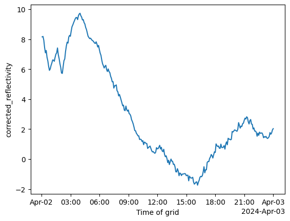
We can use xarray to get a plot of how the mean reflectivity varies by time of day, to get a general sense of how much precipitation was present in the view of the radar over time. We let xarray now to calculate the mean with respect to the spatial dimensions, leaving time.

[4]:

timeseries = radar['corrected_reflectivity'].mean(dim=['x', 'y', 'z'])

OMP: Info #276: omp_set_nested routine deprecated, please use omp_set_max_active_levels instead.

[5]:

timeseries.plot()

[5]:

[<matplotlib.lines.Line2D at 0x16ddee0d0>]

../_images/notebooks_RadarVisualisation_7_1.png

[6]:

# Select the radar data around the maximum time
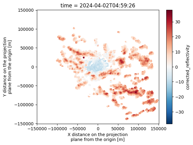
radar_at_max = radar['corrected_reflectivity'].sel({'time': '20240402T0500'}, method='nearest')

Visualising the observations#

From this time-series we can identify times when there is likely to be a good amount of precipitation in the radar observation, and choose an appropriate moment to examine the data more closely.

[7]:

radar_at_max.mean(dim='z').plot()

[7]:

<matplotlib.collections.QuadMesh at 0x16de134d0>

../_images/notebooks_RadarVisualisation_10_1.png

Visualising the radar data in three dimensions#

The above plot shows the mean average reflectivity over x and y, collapsing the vertical dimension. It tells us where rain is likely to land, but doesn’t tell us anything about the 3d-structure of the atmosphere. Visualising the data in 3D is not necessarily done often, but can be instructive. Morphological investigations are very complex!

We will need to convert the data type from the easy-to-use xarray format to a dense numpy array, as required by the visualisation library.

[8]:

# Convert the data to numpy, choosing appropriate vertical slices.
# We set aside higher vertical levels with less precipitation present
# to allow more visual emphasis on the active layers

asnumpy = radar_at_max.sel({'z': slice(500, 6000)}).round(4).fillna(0).to_numpy()

[9]:

# asnumpy.shape
# Uncomment this to determine the dimensions for the meshgrid command below

[ ]:

[10]:

# Make indexes
Z, X, Y = np.mgrid[500:6000:10j, -10:10:301j, -10:10:301j]
values = asnumpy

fig = go.Figure(
    data=go.Volume(
        x=X.flatten(),
        y=Y.flatten(),
        z=Z.flatten(),
        value=values.flatten(),
        isomin=-.99,
        isomax=0.99,
        opacity=0.01, # needs to be small to see through all surfaces
        surface_count=12, # needs to be a large number for good volume rendering,
        ),
    )

xaxis_dict = { 'title': {'text': 'Vertical distance (km)',
                         'font': {'size': 8}} }

zaxis_dict = { 'title': {'text': 'Height (m)',
                         'font': {'size': 8}} }

scene_dict = {
    'xaxis': xaxis_dict,
    'yaxis': xaxis_dict, # deliberately the same
    'zaxis': zaxis_dict,
}

fig.update_layout(
    title = "Radar reflectivity (volumetric view) - drag to rotate",
    scene_dragmode='turntable',
    autosize=False,
    width=1000,
    height=500,
    scene=scene_dict
)

fig.show()

Make sure to click and drag the plot above! It’s interactive, with an information popup if you mouse over it, and you can rotate and zoom on the data as well.

[ ]:

[ ]:

Radar Data Visualisation

Contents

Radar Data Visualisation#

Loading Data#

Time Series View#

Visualising the observations#

Visualising the radar data in three dimensions#