Train a model with the MLX framework using low hardware requirements

Train a model with the MLX framework using low hardware requirements#

This notebook uses the MLX machine learning framework and uses less than 3GB of training data. Users will need to run ‘pip install mlx’ as this is not a part of the default requirements file, as it is not available on all platforms.

Overview:

Downloading training data (takes a few minutes)
Training a neural network to predict global weather conditions (takes around 20-30 minutes per epoch)
Inferencing the network on unseen data (takes only a moment)
This tutorial demonstrates how to work with PyEarthTools using the MLX framework, which is designed for Apple Silicon.

Summary#

Choice of Data#

This tutorial allows the user to download a 2.8GB file (or 6.4GB if you choose to use additional variables). The data contains around 60 years of global Earth system analysis data. The term “analysis” means the science community’s best estimate of historical weather conditions based on available observations. The analysis data set used here was originally produced by the European Centre for Medium Range Weather Forecasting (ECMWF). This is a standard data set used in the field, however most research is done on a higher-resolution version of the data. That said, valuable research is also done using the lower resolution data. The spatial (latitude and longitude) resolution of this data is 64 pixels by 32 pixels, but the time series is very long. Only a few of the most interesting variables are downloaded in this notebook, to reduce how much data must be downloaded and stored.

The data is made available by the ECMWF under license, and the conditions are described here: https://www.ecmwf.int/en/forecasts/accessing-forecasts/licences-available . Please review this before making use of the data for anything. In this tutorial, the data is downloaded using instructions from the WeatherBench 2 data guide. Please see https://weatherbench2.readthedocs.io/en/latest/data-guide.html for more information on the data, open access, and accessing other resolutions of the data.

Defining the Neural Network#

In this notebook, we are not using PyEarthTools classes for creating a registered model or training wrapper. That would be worthwhile if the goal was to make the model itself available to a wider range of people, or encode design choices in a reference implementation that could be re-used. In this case, the goal is to show the process of neural network development directly. However, as the network is not a PyEarthTools registered model, a little bit more needs to be done after prediction to return the predictions into denormalised space as xarray objects - functionality that comes ‘for free’ with a registered model.

[6]:

class CustomGriddedRegression(nn.Module):
    """
    Create a simple five-layer network for roughly normalised regression problems
    """

    def __init__(self, num_channels, width, height):
        super().__init__()

        self.nc = num_channels
        self.w = width
        self.h = height

        self.layer1 = nn.Linear(self.nc, self.nc)
        self.layer2 = nn.Sigmoid()
        self.layer3 = nn.ReLU()
        self.layer4 = nn.Sigmoid()
        self.layer5 = nn.Linear(self.nc, self.nc)

    def __call__(self, x):
        x = self.layer1(x)
        x = self.layer2(x)
        x = self.layer3(x)
        x = self.layer4(x)
        x = self.layer5(x)
        return x

[7]:

# Here we match the size of the era5 low-resolution data. It would be interesting to experiment with larger models.
model = CustomGriddedRegression(num_channels=4, width=64, height=32)

optimizer = optim.Adam(learning_rate=0.01)

def calculate_loss(model, x, y):

    x = mx.array(x)
    y = mx.array(y)
    yhat = model(x)
    loss = nn.losses.l1_loss(yhat, y)
    return loss

def train_epoch(max_steps):
    '''
    This is be called once per epoch, and it not parameterised
    '''

    i = 0
    printper = 1000
    lossper = 0
    tic = time.perf_counter()

    # Batch size of 1 here
    for inp, tgt in data_pipeline:
        train_step_fn = nn.value_and_grad(model, calculate_loss)
        loss, grads = train_step_fn(model, inp, tgt)
        lossper += loss
        optimizer.update(model, grads)
        mx.eval(model.parameters())

        i+= 1
        if i % printper == 0:
            toc = time.perf_counter()
            average_loss = lossper / 1000
            duration = toc - tic
            print(f'Step {i}')
            print(f'Average loss over 1000 steps: {average_loss}')
            print(f'Duration for 1000 steps: {duration}')
            tic = toc
            lossper = 0

        if max_steps > 0 and i > max_steps:
            return


def do_train(epochs=1, max_steps=0):

    count_epoch = 0
    for i in range(epochs):
        print(f'Commencing epoch {i}')
        train_epoch(max_steps)
        # tr_loss, tr_acc, throughput = train_epoch(max_steps)
        # print(" | ".join([epoch, tr_loss, tr_acc, throughput]))

[8]:

# There are around 52k samples to train from
# 1000 steps was taking about 30 seconds
# So a full epoch with this model would be around 26 minutes per epoch
# Reasonable skill on this benchmark model is reached after around 6000 steps

weights_file = workdir+'/mlx_reasonable_0.safetensors'

if os.path.exists(weights_file):
    print("Loading saved model weights")
    model.load_weights(file_or_weights=weights_file)
else:
    print("Training for 10k steps - you may wish to explore additional training")
    do_train(max_steps=10000)
    model.save_weights(weights_file)

Loading saved model weights

[9]:

# do_train(max_steps=10000)

[10]:

inp, target = data_pipeline['2019-01-01']
yhat = model(mx.array(inp))

[11]:

da_pred = xr.DataArray(yhat)
da_target = xr.DataArray(target)
da_error = da_pred - da_target

[12]:

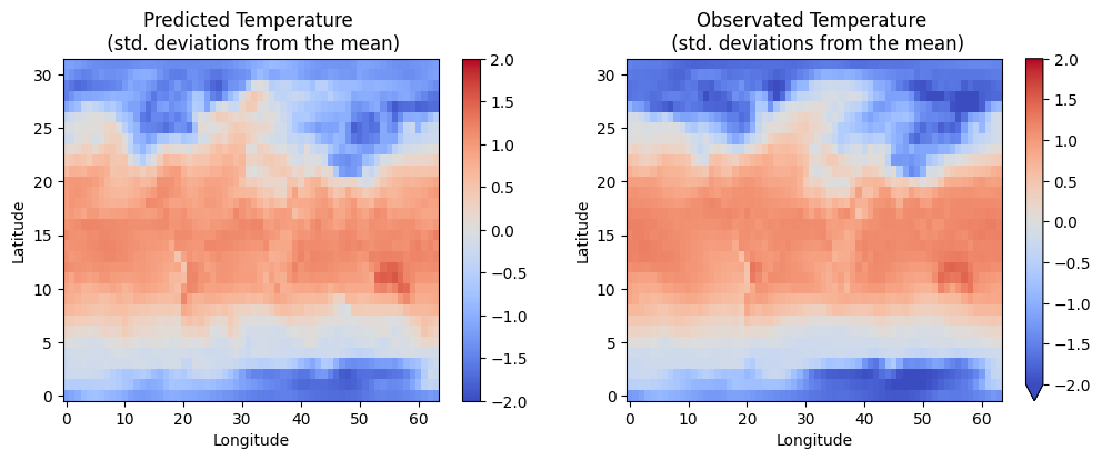
MSLP_DIM_INDEX = 2
# !NOTE! This index appears to not be the same (deterministic) on every run
# A reversible PyEarthTools Pipeline would help with keeping this consistent
# but here we are doing it from raw numpy

fig, axs = plt.subplots(ncols=2, figsize=(12, 4))
da_pred[0, :, :, MSLP_DIM_INDEX].plot(x='dim_1', y='dim_2', ax=axs[0], vmin=-2.0, vmax=2.0, cmap='coolwarm')
axs[0].set_xlabel('Longitude')
axs[0].set_ylabel('Latitude')
axs[0].set_title('Predicted Temperature \n (std. deviations from the mean)')

da_target[0, :, :, MSLP_DIM_INDEX].plot(x='dim_1', y='dim_2', ax=axs[1], vmin=-2.0, vmax=2.0, cmap='coolwarm')
axs[1].set_title('Observated Temperature \n (std. deviations from the mean)')
axs[1].set_xlabel('Longitude')
axs[1].set_ylabel('Latitude')

[12]:

Text(0, 0.5, 'Latitude')

../../_images/notebooks_tutorial_MLX-Demo-Custom-Arch_13_1.png

[ ]:

Train a model with the MLX framework using low hardware requirements

Contents

Train a model with the MLX framework using low hardware requirements#

Summary#

Choice of Data#

Note on the MLX Framework#

Defining the Neural Network#