HadISD Tutorial Five - Integration of Station Data with PyEarthTools#
NOTE Before beginning this tutorial, you should first read HadISD Tutorial One - Introduction to Station Data and ensure you complete the tutorials in order
This tutorial demonstrates how to create a data accessor for the station data which will integrate with PyEarthTools pipelines. In due course, a similar implementation will be put into the relevant site archive packages for people working in supported facilities, but this demonstrates how you can easily connect your own station data archive into the framework from first principles. Working with custom station datasets is relatively common (e.g. hydrology-specific data sets, different temporal resolutions, region-specific datasets, data sources not included in the global data sharing etc) and so seeing the entire process is of value.
This tutorial will show how to:
Create a data accessor on-the-fly in the notebook
Access and plot data
Access that data alongside gridded data, and plot the overlay
Note! The data visualised in this notebook is only showing a small subset of the total number of stations, as it was developed on limited data in the first instance. Tutorials six and seven demonstrate the use of all stations based on the much faster Parquet storage format.
[1]:
import pyearthtools.data
import pyearthtools.pipeline
from pyearthtools.data import Petdt

from pathlib import Path
DECADAL_DIR = Path('/g/data/kd24/data') / 'hadisd' / 'by_decade'
WBERA5_DIR = Path('/g/data/kd24/data') / 'wbera5' / 'by_decade'

from mpl_toolkits.basemap import Basemap
[2]:
from pyearthtools.data.archive import register_archive
from pyearthtools.data.exceptions import DataNotFoundError
from pyearthtools.data.indexes import ArchiveIndex, decorators
from pyearthtools.data.transforms import Transform, TransformCollection
import xarray as xr
import numpy as np

@register_archive("ISD", sample_kwargs=dict(variable="2t"))
class ISD(ArchiveIndex):
    @property
    def _desc_(self):
        return {
            "singleline": "Hadley Integrated Surface Database",
            "range": "1930 - 2025",
            "Documentation": "https://www.metoffice.gov.uk/hadobs/hadisd/",
        }

    def __init__(
        self,
        disk_location,
        *,
        transforms: Transform | TransformCollection | None = None,
    ):

        self.disk_location = Path(disk_location)  # Location of the large groupings files
        super().__init__(transforms=transforms or TransformCollection())

    def filesystem(self, querytime: str | Petdt):
        '''
        This is quick, no need to cache it
        '''
        files = list(self.disk_location.glob('*1990*.nc'))
        return files

    def load(self, from_files_list, **kwargs):

        ds = xr.open_mfdataset(from_files_list, combine='nested', concat_dim='report')

        # Arguably, this should be a transform, or handled in the pipeline, but it works for now
        ds['temperatures'] = ds.temperatures.where(ds.temperatures > -1000)
        return ds
[3]:
era5_source = pyearthtools.data.download.weatherbench.WB2ERA5(
        variables=["2m_temperature", "u", "v", "geopotential"],
        level=[850],
        download_dir=WBERA5_DIR,
        license_ok=True,
    ),

station_source = ISD(DECADAL_DIR)

data_pipeline = pyearthtools.pipeline.Pipeline(
    (era5_source, station_source)
)
[4]:
# Here we see the pipeline returns the ERA5 grid and the station data as two separate datasets, at a matched time.
data_pipeline['19900620T00']
[4]:
(<xarray.Dataset> Size: 34kB
 Dimensions:              (time: 1, longitude: 64, latitude: 32, level: 1)
 Coordinates:
   * time                 (time) datetime64[ns] 8B 1990-06-20
   * longitude            (longitude) float64 512B 0.0 5.625 ... 348.8 354.4
   * latitude             (latitude) float64 256B -87.19 -81.56 ... 81.56 87.19
   * level                (level) int64 8B 850
 Data variables:
     2m_temperature       (time, longitude, latitude) float32 8kB dask.array<chunksize=(1, 64, 32), meta=np.ndarray>
     u_component_of_wind  (time, level, longitude, latitude) float32 8kB dask.array<chunksize=(1, 1, 64, 32), meta=np.ndarray>
     v_component_of_wind  (time, level, longitude, latitude) float32 8kB dask.array<chunksize=(1, 1, 64, 32), meta=np.ndarray>
     geopotential         (time, level, longitude, latitude) float32 8kB dask.array<chunksize=(1, 1, 64, 32), meta=np.ndarray>,
 <xarray.Dataset> Size: 17MB
 Dimensions:                (time: 1, report: 50, test: 71, flagged: 19,
                             reporting_v: 19, reporting_t: 1140, reporting_2: 2)
 Coordinates:
   * time                   (time) datetime64[ns] 8B 1990-06-20
 Dimensions without coordinates: report, test, flagged, reporting_v,
                                 reporting_t, reporting_2
 Data variables: (12/30)
     station_id             (time, report) |S12 600B dask.array<chunksize=(1, 50), meta=np.ndarray>
     temperatures           (time, report) float64 400B dask.array<chunksize=(1, 25), meta=np.ndarray>
     dewpoints              (time, report) float64 400B dask.array<chunksize=(1, 25), meta=np.ndarray>
     slp                    (time, report) float64 400B dask.array<chunksize=(1, 25), meta=np.ndarray>
     stnlp                  (time, report) float64 400B dask.array<chunksize=(1, 25), meta=np.ndarray>
     windspeeds             (time, report) float64 400B dask.array<chunksize=(1, 25), meta=np.ndarray>
     ...                     ...
     quality_control_flags  (time, report, test) float64 28kB dask.array<chunksize=(1, 8, 12), meta=np.ndarray>
     flagged_obs            (time, report, flagged) float64 8kB dask.array<chunksize=(1, 13, 4), meta=np.ndarray>
     reporting_stats        (time, report, reporting_v, reporting_t, reporting_2) float64 17MB dask.array<chunksize=(1, 50, 19, 1140, 2), meta=np.ndarray>
     lat                    (time, report) float64 400B dask.array<chunksize=(1, 50), meta=np.ndarray>
     lon                    (time, report) float64 400B dask.array<chunksize=(1, 50), meta=np.ndarray>
     elev                   (time, report) float64 400B dask.array<chunksize=(1, 50), meta=np.ndarray>)
[5]:
grid, points = data_pipeline['19900620T00']
[6]:
# Transform gridded data for plotting
lats = grid['latitude'].values
lons = grid['longitude'].values
data = grid['2m_temperature'].values[0]  # Replace with your variable name
lon, lat = np.meshgrid(lons, lats)
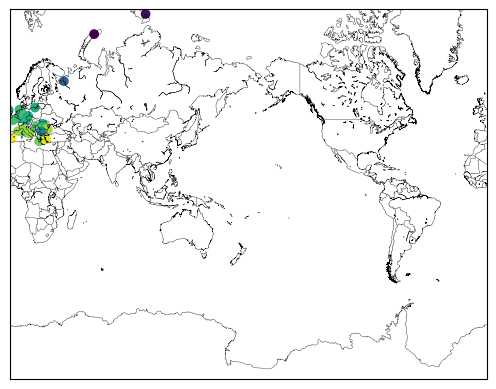
[7]:
# First, just plot the station data so we can see where our data subset is

map = Basemap(projection='merc',llcrnrlat=-80,urcrnrlat=80,\
            llcrnrlon=0,urcrnrlon=360,lat_ts=20,resolution='l')
# draw coastlines, country boundaries, fill continents.
map.drawcoastlines(linewidth=0.25)
map.drawcountries(linewidth=0.25)

# # Add station data over the top
x2, y2 = map(points.lon, points.lat)

map.scatter(x2, y2, c=points.temperatures, cmap='viridis')
[7]:
<matplotlib.collections.PathCollection at 0x14b7b4bc1990>
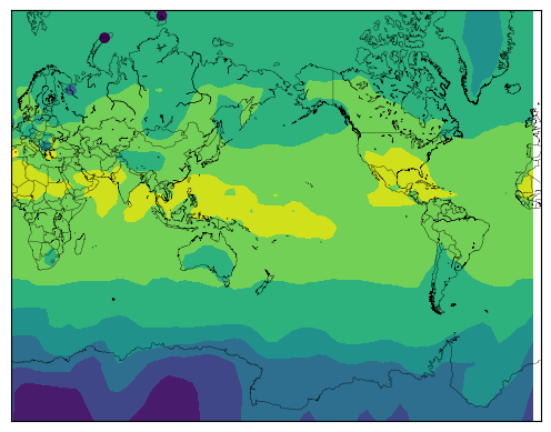
[8]:
# Then, plot the stations over the gridded data to see the overlay

map = Basemap(projection='merc',llcrnrlat=-80,urcrnrlat=80,\
            llcrnrlon=0,urcrnrlon=360,lat_ts=20,resolution='l')
# draw coastlines, country boundaries, fill continents.
map.drawcoastlines(linewidth=0.25)
map.drawcountries(linewidth=0.25)

x, y = map(lon, lat)


# # Add station data over the top
x2, y2 = map(points.lon, points.lat)

map.contourf(x, y, data.T, cmap='viridis')
map.scatter(x2, y2, c=points.temperatures, cmap='viridis')
[8]:
<matplotlib.collections.PathCollection at 0x14b7b433f2d0>
[ ]:
[ ]: