Tutorial: ENSO Pipeline#
This notebook shows how the data preprocessing steps performed in the ENSO_Forecast notebook can be replicated using the built-in PyEarthTools pipeline.
The purpose is to use the PyEarthTools pipeline to:
load ERA5 global data,
crop the data within the Nino3.4 spatial domain, and
calculate the spatial mean for each time step.
This pipeline is applied to ERA5 monthly temperature data. The next step is to calculate the Nino3.4 time series.
[4]:
# Necessary import
import pyearthtools.data
import pyearthtools.pipeline as petpipe
import site_archive_nci
import warnings
import xarray as xr
#import plotly.express as px
import matplotlib.pyplot as plt
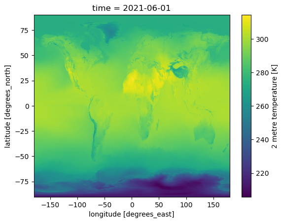
Load and process ERA5 2-metre air temperature (t2m) data. We want to calculate the Niño3.4 index from the t2m anomalies in the region 5°N–5°S, 170°W–120°W.#
[5]:
# Total time frame for training the model
start = '1970-01-01'
end = '2024-12-31'

# Start by considering a specific date for visualising the process on one sample
doi = '2021-06-09T06' # Note - if you change 'product' to 'reanalysis' you can get the 6-hour timesteps
variables_of_interest = ['2t']
product = 'monthly-averaged'
accessor = pyearthtools.data.archive.ERA5(variables_of_interest, product=product)
accessor[doi][variables_of_interest[0]].plot()
/opt/conda/envs/pet/lib/python3.11/site-packages/pyearthtools/data/indexes/_indexes.py:809: IndexWarning: Data requested at a higher resolution than available. hour > month
  warnings.warn(
[5]:
<matplotlib.collections.QuadMesh at 0x1507c9d2dad0>
[6]:
min_lat = -5
max_lat = 5
min_lon = -170
max_lon = -120

# Helper transform to compute the spatial mean
class PointMean(pyearthtools.data.transforms.Transform):

    def apply(self, dataset, **kwargs):
       # dataset['2t'] = dataset['2t'].mean(dim=['latitude', 'longitude'])
        dataset[variables_of_interest[0]] = dataset[variables_of_interest[0]].mean(dim=['latitude', 'longitude'])
        return dataset


# Perform the preprocessing steps in one pipeline: load, crop, and average
pipeline = petpipe.Pipeline(
    accessor,
    pyearthtools.data.transform.region.Bounding(min_lat, max_lat, min_lon, max_lon), # keep only data within the bounding box
    PointMean(), # Calculate spatial mean
    sampler=pyearthtools.pipeline.samplers.Default(),
    iterator=pyearthtools.pipeline.iterators.DateRange(start, end, interval='1 month')     # Retrieve monthly data from 1970 to the end of 2024
)
pipeline
Pipeline
    Description                    `pyearthtools.pipeline` Data Pipeline


    Initialisation
             exceptions_to_ignore           None
             iterator                       {'DateRange': {'allowlist': 'None', 'blocklist': 'None', 'end': "'2024-12-31'", 'interval': "'1 month'", 'start': "'1970-01-01'"}}
             sampler                        {'Default': {}}
    Steps
             ERA5                           {'ERA5': {'level_value': 'None', 'product': "'monthly-averaged'", 'variables': "['2t']"}}
             region.Bounding                {'Bounding': {'max_lat': '5', 'max_lon': '-120', 'min_lat': '-5', 'min_lon': '-170'}}
__main__.PointMean {'PointMean': {}}Graph

[3]:
%%time
# Takes around ten seconds
all_steps = None
with warnings.catch_warnings():
    warnings.simplefilter("ignore") # suppress warnings during pipeline execution
    all_steps = list(pipeline) # execute the pipeline and store all results in a list
CPU times: user 11.6 s, sys: 1.78 s, total: 13.4 s
Wall time: 43 s
[9]:
# extract the '2t' variable (variable of interest) from each pipeline output
all_temps = [s[variables_of_interest[0]] for s in all_steps]

# concatenate all temperature datasets along the time dimension
ds = xr.concat(all_temps, dim='time')
[10]:
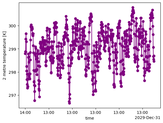
# plot the time series
ds.plot.line(color="purple", marker="o")
[10]:
[<matplotlib.lines.Line2D at 0x1507ba420f50>]
Next, you can replicate the steps in ENSO_Forecast notebook from 4. Calculate the Niño3.4 index onward.#
[12]:
# Convert to pandas DataFrame with 3 columns 'year' 'month' and 't2m' (i.e. 2t timeseries)
df = ds.to_dataframe(name='t2m').reset_index()

# Extract year and month from 'time'
df['year'] = df['time'].dt.year
df['month'] = df['time'].dt.month

# Keep required columns
t2_df = df[['year', 'month', 't2m']]

print("\nPrinting first 10 rows of t2_df:")
t2_df.head(10)
Printing first 10 rows of t2_df:
[12]:
| year | month | t2m | |
|---|---|---|---|
| 0 | 1970 | 1 | 298.799964 |
| 1 | 1970 | 2 | 298.884142 |
| 2 | 1970 | 3 | 298.863824 |
| 3 | 1970 | 4 | 299.425736 |
| 4 | 1970 | 5 | 299.650770 |
| 5 | 1970 | 6 | 299.316589 |
| 6 | 1970 | 7 | 298.237027 |
| 7 | 1970 | 8 | 298.046338 |
| 8 | 1970 | 9 | 297.680157 |
| 9 | 1970 | 10 | 297.906577 |
Calculate the Niño3.4 index#
[14]:
# Calculate monthly climatology
monthly_clim = t2_df.groupby('month')['t2m'].mean()
print("Printing monthly climatology (mean t2m by month):")
monthly_clim

# Assign the climatology value to each row
t2_df['monthly_clim'] = t2_df['month'].map(monthly_clim)

# Calculate monthly anomalies
t2_df['anom'] = t2_df['t2m'] - t2_df['monthly_clim']

# Minus 5-year moving average to remove trend
t2_df['anom_detrended'] = t2_df['anom'] - t2_df['anom'].rolling(window=60, center=True, min_periods=1).mean()

# Apply 5 month running average
t2_df['anom_smoothed'] = t2_df['anom_detrended'].rolling(window=5, center=True, min_periods=1).mean()

# Normalise by the standard deviation of the time series
std_val = t2_df['anom_smoothed'].std()
t2_df['nino3.4'] = t2_df['anom_smoothed'] / std_val

print("\nPrinting first 10 rows of t2_df:")
t2_df.head(10)
Printing monthly climatology (mean t2m by month):

Printing first 10 rows of t2_df:
[14]:
| year | month | t2m | monthly_clim | anom | anom_detrended | anom_smoothed | nino3.4 | |
|---|---|---|---|---|---|---|---|---|
| 0 | 1970 | 1 | 298.799964 | 298.664784 | 0.135180 | 0.797918 | 0.568150 | 0.885935 |
| 1 | 1970 | 2 | 298.884142 | 298.846780 | 0.037362 | 0.653045 | 0.515593 | 0.803981 |
| 2 | 1970 | 3 | 298.863824 | 299.178853 | -0.315029 | 0.253487 | 0.496437 | 0.774111 |
| 3 | 1970 | 4 | 299.425736 | 299.585783 | -0.160047 | 0.357922 | 0.371018 | 0.578540 |
| 4 | 1970 | 5 | 299.650770 | 299.701533 | -0.050762 | 0.419813 | 0.114479 | 0.178510 |
| 5 | 1970 | 6 | 299.316589 | 299.568230 | -0.251641 | 0.170821 | -0.045365 | -0.070739 |
| 6 | 1970 | 7 | 298.237027 | 299.242830 | -1.005803 | -0.629650 | -0.278800 | -0.434741 |
| 7 | 1970 | 8 | 298.046338 | 298.925642 | -0.879304 | -0.545729 | -0.470833 | -0.734185 |
| 8 | 1970 | 9 | 297.680157 | 298.792747 | -1.112591 | -0.809253 | -0.699846 | -1.091294 |
| 9 | 1970 | 10 | 297.906577 | 298.731676 | -0.825098 | -0.540353 | -0.793144 | -1.236776 |
[ ]: